GITT analysis
In this notebook we will use cellpy to extract the open circuit voltages (OCV) from a GITT measurement. The extracted OCVs will be plotted, and the results saved in .csv format."
import pathlib
import pandas as pd
import matplotlib.pyplot as plt

import cellpy
from cellpy.utils import plotutils
Set filepath and load the datafile:
filedir = pathlib.Path("data")  # foldername within the same directory
c = cellpy.get(filedir / "out" / "20210210_FC.h5")
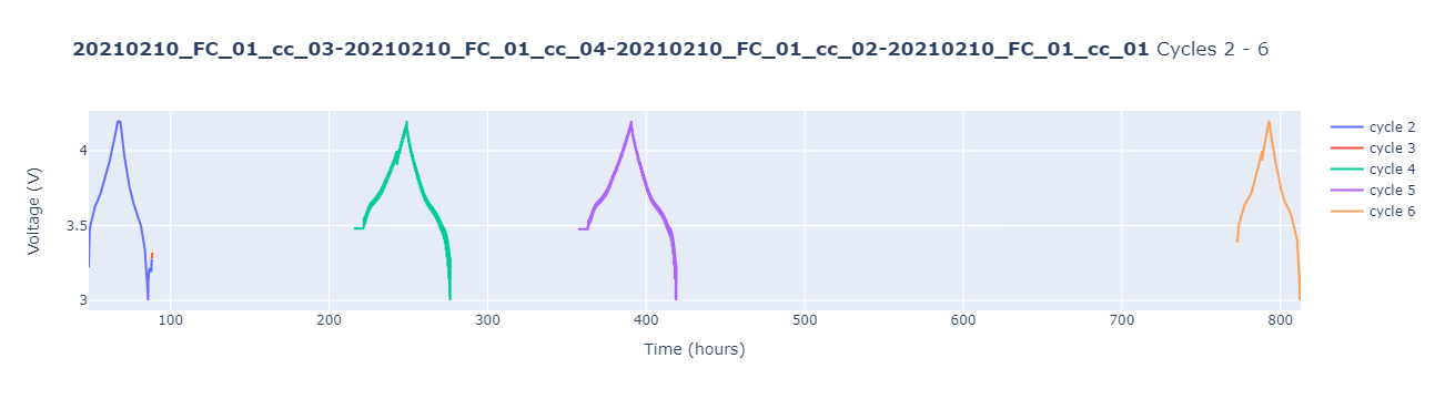
Produce an overview plot to identify cycle numbers for the GITT experiment (for an interactive version of this plot, you have to have plotly installed):
OCV extraction
From the overview plot above, we can identify the GITT cycles to be cycle number 4 and 5. In the following, we will focus on cycle 5 only.
For further analysis, we create the step table, called steps, a dataframe that contains a lot ofnformation on all the cycle steps for the cell.
In the following, we apply several filters to steps, to eventually extract OCV voltages and corresponding capacities:
steps_cycle: Extract the rows specifically for the selected GITT cycle (here: cycle Nr 5).
NB: For simplicity, steps_cycle only contains rows relevant for further analysis, i.e. "cycle", "step""charge_last", "discharge_last", "voltage_first" ,"voltage_last", "type"."
GITT_cycle = 5
c.make_step_table(all_steps=True)
steps = c.data.steps
steps_cycle = steps.loc[
    (steps.cycle == GITT_cycle),
    [
        "cycle",
        "step",
        "charge_last",
        "discharge_last",
        "voltage_first",
        "voltage_last",
        "type",
    ],
]
Taking a closer look at the created steps_cycle dataframe:
steps_cycle.head(10)to view the first 10 rowssteps_cycle.tail(10)to view the last 10 rows
     cycle  step  charge_last  discharge_last  voltage_first  voltage_last  \
755      5     8     0.003358        0.003258       3.212396      3.343531
756      5     7     0.003358        0.003294       3.330632      3.139919
757      5     8     0.003358        0.003294       3.162645      3.314970
758      5     7     0.003358        0.003330       3.302993      3.080647
759      5     8     0.003358        0.003330       3.102759      3.283338
760      5     7     0.003358        0.003366       3.272282      3.008170
761      5     8     0.003358        0.003366       3.029361      3.246485
762      5     7     0.003358        0.003392       3.233587      2.999878
763      5    10     0.003358        0.003392       3.010627      3.010627
764      5    11     0.003358        0.003392       3.037038      3.228980

          type
755  ocvrlx_up
756  discharge
757  ocvrlx_up
758  discharge
759  ocvrlx_up
760  discharge
761  ocvrlx_up
762  discharge
763         ir
764  ocvrlx_up
- To extract the OCV voltages, we then filter the
steps_cycledataframe for- the OCV relaxation steps on discharge,
steps_ocv_dch, of type oxvrlx_up (and rest), corresponding tostep==3, and - the OCV relaxation steps on charge
steps_ocv_cha, of type oxvrlx_down (and rest), corresponding tostep==8. Thereby we obtain two new dataframes
- the OCV relaxation steps on discharge,
steps_ocv_cha = steps_cycle.loc[steps_cycle.step == 3]
steps_ocv_dch = steps_cycle.loc[steps_cycle.step == 8]
     cycle  step  charge_last  discharge_last  voltage_first  voltage_last  \
390      5     3     0.000036             0.0       3.512440      3.487564
392      5     3     0.000072             0.0       3.518582      3.494320
394      5     3     0.000109             0.0       3.524724      3.499848
396      5     3     0.000145             0.0       3.530559      3.505991
398      5     3     0.000181             0.0       3.537315      3.513054

     type
390  rest
392  rest
394  rest
396  rest
398  rest
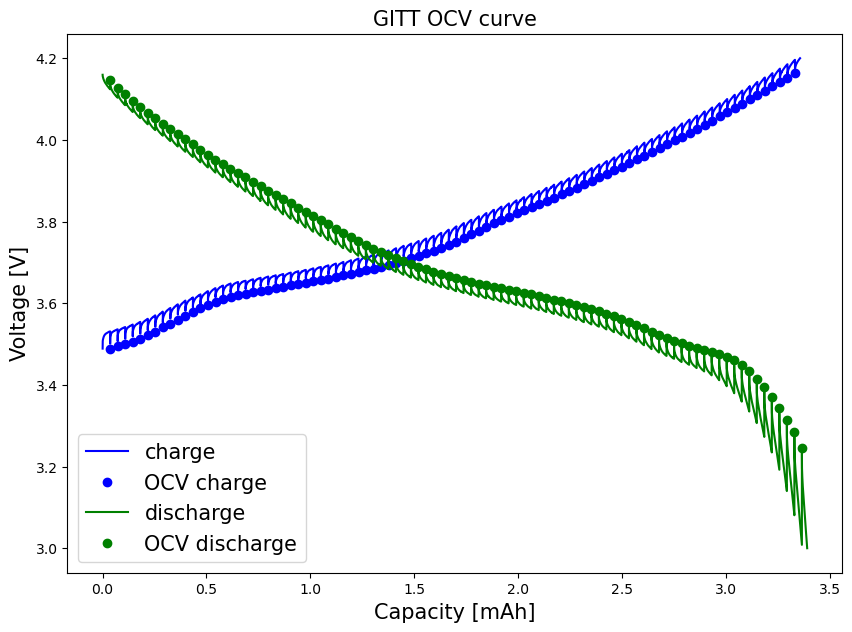
The voltages at the end of these steps (voltage_last), contain the (pseudo-) OCV voltages:
V_cha = steps_ocv_cha.voltage_last.reset_index(drop=True)
V_dch = steps_ocv_dch.voltage_last.reset_index(drop=True)
cap_cha = (
    steps_ocv_cha.charge_last.reset_index(drop=True) * 1000
)  # *1000 to convert to mAh
cap_dch = (
    steps_ocv_dch.discharge_last.reset_index(drop=True) * 1000
)  # *1000 to convert to mAh
To plot our results, we additionally get the entire voltage vs capacity curves for the selected GITT cycle, employing the .get_ccap and .get_dcap methods. The cell mass is used to convert from gravimetric capacity (mAh/g) to capacity (mAh).
c.make_step_table(all_steps=False)
ccap = c.get_ccap(cycle=GITT_cycle)
dcap = c.get_dcap(cycle=GITT_cycle)
mass = c.get_mass()  # in mg
fig, ax = plt.subplots()
ax.plot(
    ccap["charge_capacity"] * mass / 1000, ccap["voltage"], color="blue", label="charge"
)
ax.plot(cap_cha, V_cha, "bo", label="OCV charge")
ax.plot(
    dcap["discharge_capacity"] * mass / 1000,
    dcap["voltage"],
    color="green",
    label="discharge",
)
ax.plot(cap_dch, V_dch, "go", label="OCV discharge")
plt.xlabel("Capacity [mAh]", fontsize=15)
plt.ylabel("Voltage [V]", fontsize=15)
plt.title("GITT OCV curve", fontsize=15)
# plt.ylim(0, 0.91)
# plt.xlim(0, 4.70)
ax.legend(fontsize=15)
fig.set_figheight(7)
fig.set_figwidth(10)
plt.show()
Saving the data
Concatenate the OCV voltages and capacities into a dataframe, and save as a .csv file.