Initial data inspection and plotting
Hint
If you have plotly installed, some of the functions will produce interactive plots. If not, the output will be simpler matplotlib figures. If you have not installed plotly, you can do so by running pip install plotly.
Either load raw data or your saved cellpy files:
filedir = pathlib.Path("data")  # foldername within the same directory
c = cellpy.get(filedir / "out" / "20210210_FC.h5")
Looking at the data
Your CellpyCell object (here called c) contains all your raw data as well as some additional elements, in the format of pandas DataFrames:
- Raw data:
c.data.raw, raw data from the run (with unitsc.data.raw_units) - Summary:
c.data.summarywith cycle-based summaries - Steps:
c.data.stepswith Stats from each step (and step type), created using thec.make_step_tablemethod
            test_id  data_point  test_time  step_time           date_time  \
data_point
1                 1           1   5.008961   5.008961 2021-05-10 10:14:45
2                 1           2  10.019319  10.019319 2021-05-10 10:14:50

            step_index  cycle_index  is_fc_data  current   voltage  \
data_point
1                    1            1           0      0.0  3.051165
2                    1            1           0      0.0  3.051165

            charge_capacity  discharge_capacity  charge_energy  \
data_point
1                       0.0                 0.0            0.0
2                       0.0                 0.0            0.0

            discharge_energy     dv_dt  internal_resistance  ac_impedance  \
data_point
1                        0.0 -0.000061                  0.0           0.0
2                        0.0  0.000000                  0.0           0.0

            aci_phase_angle
data_point
1                       0.0
2                       0.0
             data_point      test_time           date_time  \
cycle_index
1                  5797  174328.601353 2021-05-12 10:40:11
2                  7188  317161.773416 2021-05-14 02:20:47

             end_voltage_charge  end_voltage_discharge  charge_capacity  \
cycle_index
1                      4.200052               3.129170         0.003819
2                      4.200052               3.188442         0.003422

             discharge_capacity  coulombic_efficiency  \
cycle_index
1                      0.003324             87.049469
2                      0.003234             94.510786

             cumulated_coulombic_efficiency  cumulated_charge_capacity  ...  \
cycle_index                                                             ...
1                                 87.049469                   0.003819  ...
2                                181.560255                   0.007241  ...

             cumulated_charge_capacity_areal  \
cycle_index
1                                   3.818560
2                                   7.240795

             cumulated_discharge_capacity_areal  coulombic_difference_areal  \
cycle_index
1                                      3.324036                    0.494524
2                                      6.558417                    0.187854

             cumulated_coulombic_difference_areal  \
cycle_index
1                                        0.494524
2                                        0.682378

             discharge_capacity_loss_areal  charge_capacity_loss_areal  \
cycle_index
1                                      NaN                         NaN
2                                 0.089654                    0.396324

             cumulated_discharge_capacity_loss_areal  \
cycle_index
1                                                NaN
2                                           0.089654

             cumulated_charge_capacity_loss_areal  \
cycle_index
1                                             NaN
2                                        0.396324

             shifted_charge_capacity_areal  shifted_discharge_capacity_areal
cycle_index
1                                 0.494524                          4.313083
2                                 0.682378                          4.104613

[2 rows x 49 columns]
   index  cycle  step  sub_step  point_avr   point_std  point_min  point_max  \
0      0      1     1         1     2157.5  1245.48886          1       4314
1      1      1     2         1     4315.0         NaN       4315       4315

   point_first  point_last  ...  ir_std    ir_min    ir_max  ir_first  \
0            1        4314  ...     0.0  0.000000  0.000000  0.000000
1         4315        4315  ...     NaN  6.650723  6.650723  6.650723

    ir_last  ir_delta  rate_avr  type  sub_type  info
0  0.000000       0.0   0.00000  rest       NaN
1  6.650723       0.0   1.75791    ir       NaN

[2 rows x 64 columns]
Simple plotting
The plotutils module contains several convenient plot functions:
Raw plots
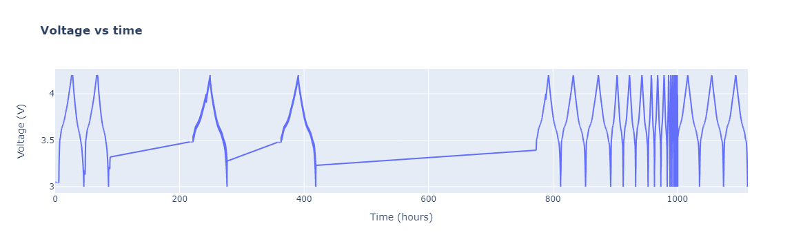
The raw_plot gives an overview of your datacollection, plotting voltage vs time:
Cycle info plots
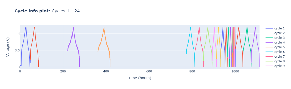
The cycle_info_plot function plots the raw data together with step and cycle info:
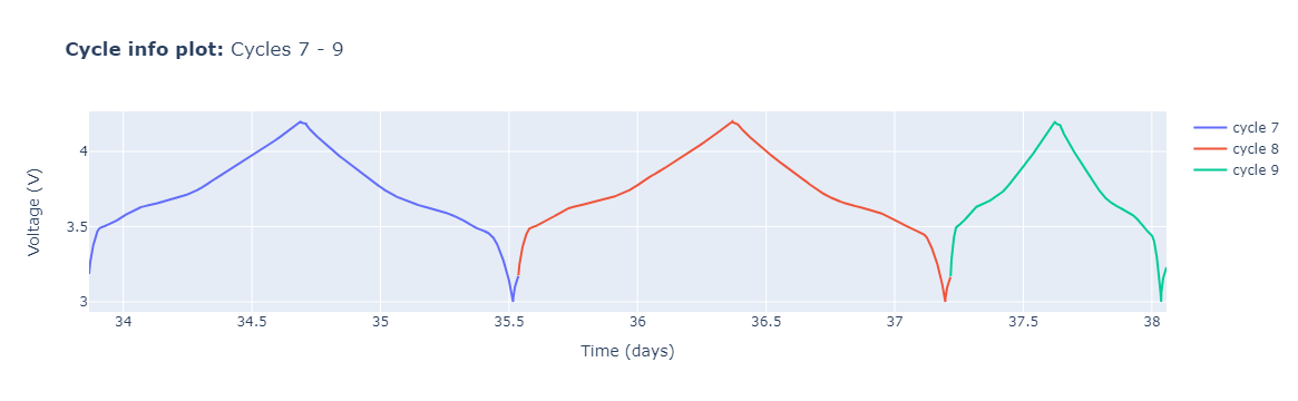
These plot functions offer some flexibility. You can, e.g. select specific cycles to look at, or adjust the units of the plot variables:
Summary plots
summary_plots allows you to plot different summary variables. You can inspect the columns of c.data.summary to check what variables are available.
Index(['data_point', 'test_time', 'date_time', 'end_voltage_charge',
       'end_voltage_discharge', 'charge_capacity', 'discharge_capacity',
       'coulombic_efficiency', 'cumulated_coulombic_efficiency',
       'cumulated_charge_capacity', 'cumulated_discharge_capacity',
       'discharge_capacity_loss', 'charge_capacity_loss',
       'coulombic_difference', 'cumulated_coulombic_difference',
       'cumulated_discharge_capacity_loss', 'cumulated_charge_capacity_loss',
       'shifted_charge_capacity', 'shifted_discharge_capacity',
       'cumulated_ric', 'cumulated_ric_sei', 'cumulated_ric_disconnect',
       'normalized_cycle_index', 'charge_c_rate', 'discharge_c_rate',
       'discharge_capacity_gravimetric', 'charge_capacity_gravimetric',
       'cumulated_charge_capacity_gravimetric',
       'cumulated_discharge_capacity_gravimetric',
       'coulombic_difference_gravimetric',
       'cumulated_coulombic_difference_gravimetric',
       'discharge_capacity_loss_gravimetric',
       'charge_capacity_loss_gravimetric',
       'cumulated_discharge_capacity_loss_gravimetric',
       'cumulated_charge_capacity_loss_gravimetric',
       'shifted_charge_capacity_gravimetric',
       'shifted_discharge_capacity_gravimetric', 'discharge_capacity_areal',
       'charge_capacity_areal', 'cumulated_charge_capacity_areal',
       'cumulated_discharge_capacity_areal', 'coulombic_difference_areal',
       'cumulated_coulombic_difference_areal', 'discharge_capacity_loss_areal',
       'charge_capacity_loss_areal', 'cumulated_discharge_capacity_loss_areal',
       'cumulated_charge_capacity_loss_areal', 'shifted_charge_capacity_areal',
       'shifted_discharge_capacity_areal'],
      dtype='object')
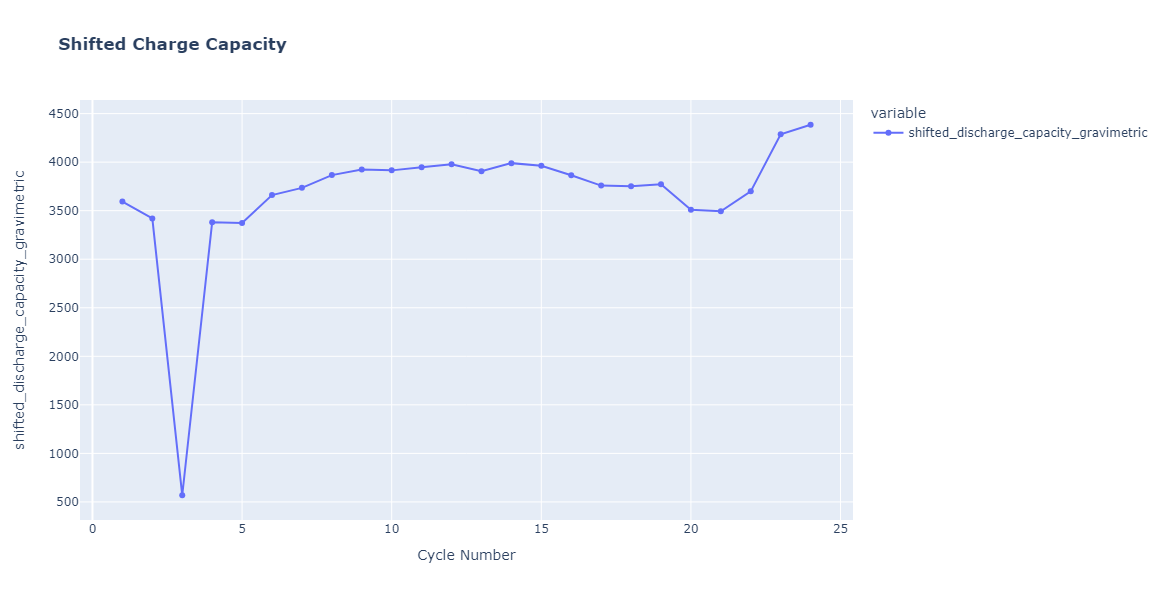
Here is one example:
plotutils.summary_plot(
    c,
    y="shifted_discharge_capacity_gravimetric",
    title="<b>Shifted Charge Capacity</b>",
)
The summary_plot function also have some pre-defined sets of variables for plotting the most common variables.
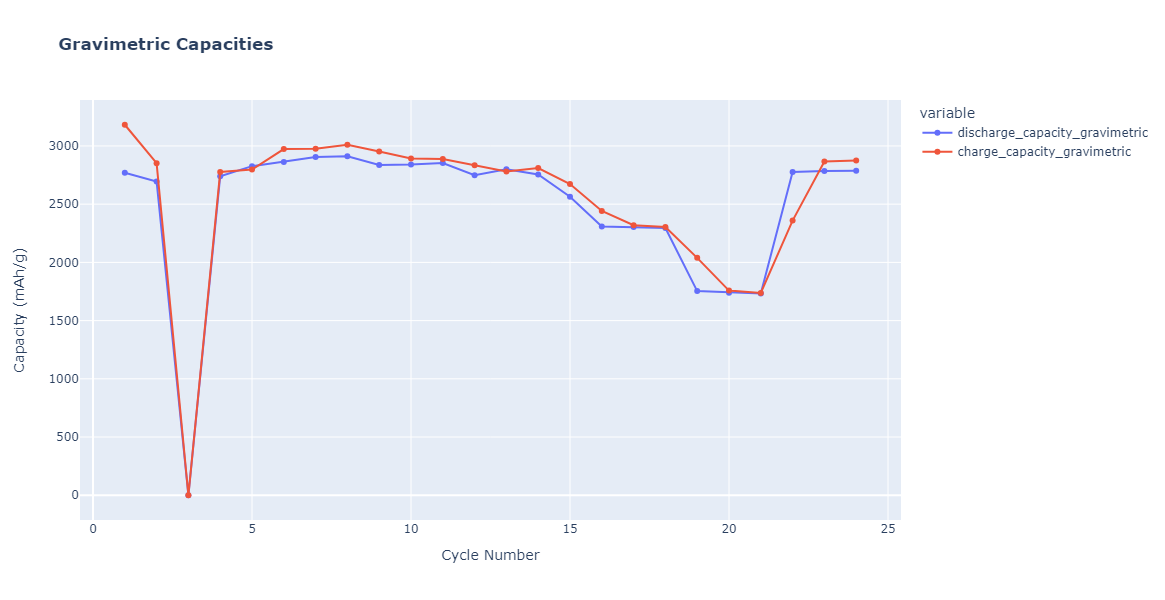
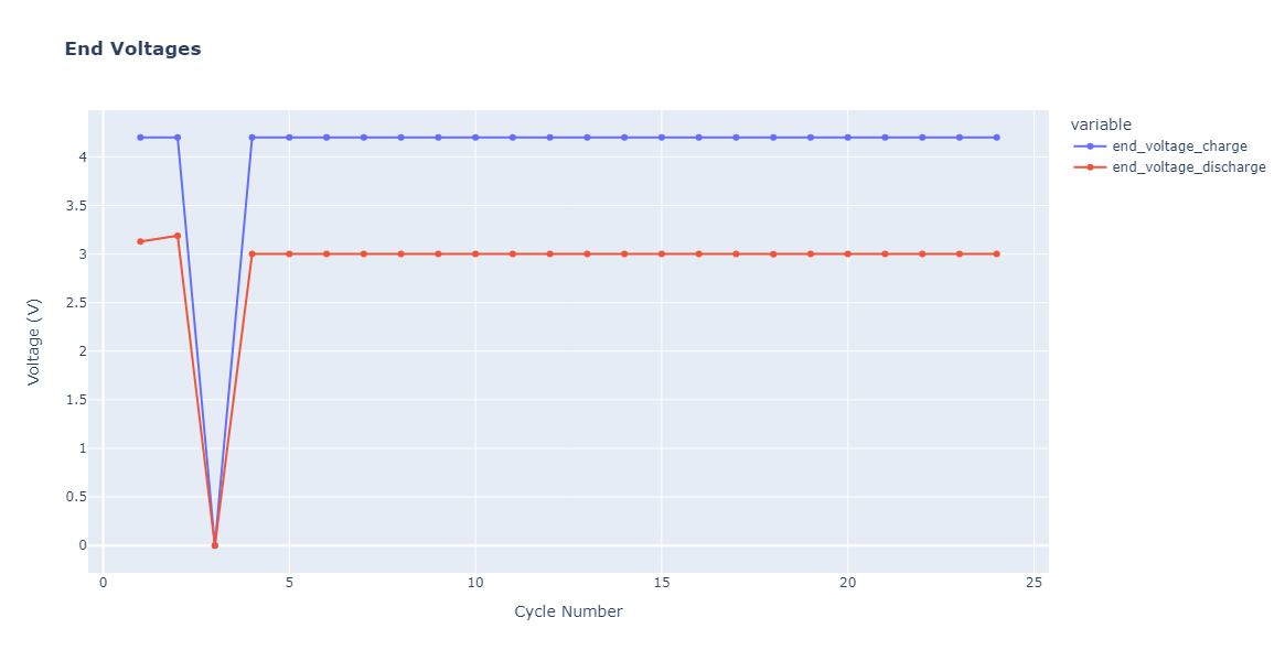
The pre-defined variable sets for the summary plots are: - "voltages" - "capacities_gravimetric" - "capacities_areal" - "capacities_gravimetric_split_constant_voltage" - "capacities_areal_split_constant_voltage"