GITT analysis

In this notebook we will use cellpy to extract the open circuit voltages (OCV) from a GITT measurement. The extracted OCVs will be plotted, and the results saved in .csv format.”

import pathlib
import pandas as pd
import matplotlib.pyplot as plt

import cellpy
from cellpy.utils import plotutils

Set filepath and load the datafile:

filedir=pathlib.Path("data") # foldername within the same directory
c = cellpy.get(filedir / 'out' / '20210210_FC.h5')

Produce an overview plot to identify cycle numbers for the GITT experiment (for an interactive version of this plot, you have to have plotly installed):

plotutils.cycle_info_plot(c, cycle = list(range(2, 7)))

OCV extraction

From the overview plot above, we can identify the GITT cycles to be cycle number 4 and 5. In the following, we will focus on cycle 5 only.

For further analysis, we create the step table, called steps, a dataframe that contains a lot ofnformation on all the cycle steps for the cell.

In the following, we apply several filters to steps, to eventually extract OCV voltages and corresponding capacities:

1. ``steps_cycle``: Extract the rows specifically for the selected GITT cycle (here: cycle Nr 5).

NB: For simplicity, steps_cycle only contains rows relevant for further analysis, i.e. “cycle”, “step””charge_last”, “discharge_last”, “voltage_first” ,”voltage_last”, “type”.”

GITT_cycle=5
c.make_step_table(all_steps=True)
steps=c.data.steps
steps_cycle=steps.loc[(steps.cycle==GITT_cycle),["cycle", "step", "charge_last", "discharge_last", "voltage_first" ,"voltage_last", "type"]]

Taking a closer look at the created steps_cycle dataframe:

• steps_cycle.head(10) to view the first 10 rows

• steps_cycle.tail(10) to view the last 10 rows

steps_cycle.tail(10)

	cycle	step	charge_last	discharge_last	voltage_first	voltage_last	type
755	5	8	0.003358	0.003258	3.212396	3.343531	ocvrlx_up
756	5	7	0.003358	0.003294	3.330632	3.139919	discharge
757	5	8	0.003358	0.003294	3.162645	3.314970	ocvrlx_up
758	5	7	0.003358	0.003330	3.302993	3.080647	discharge
759	5	8	0.003358	0.003330	3.102759	3.283338	ocvrlx_up
760	5	7	0.003358	0.003366	3.272282	3.008170	discharge
761	5	8	0.003358	0.003366	3.029361	3.246485	ocvrlx_up
762	5	7	0.003358	0.003392	3.233587	2.999878	discharge
763	5	10	0.003358	0.003392	3.010627	3.010627	ir
764	5	11	0.003358	0.003392	3.037038	3.228980	ocvrlx_up

2. To extract the OCV voltages, we then filter the steps_cycle dataframe for

   • the OCV relaxation steps on discharge, steps_ocv_dch, of type oxvrlx_up (and rest), corresponding to step==3, and

   • the OCV relaxation steps on charge steps_ocv_cha, of type oxvrlx_down (and rest), corresponding to step==8. Thereby we obtain two new dataframes

steps_ocv_cha = steps_cycle.loc[steps_cycle.step==3]
steps_ocv_dch = steps_cycle.loc[steps_cycle.step==8]

steps_ocv_cha.head(5)

	cycle	step	charge_last	discharge_last	voltage_first	voltage_last	type
390	5	3	0.000036	0.0	3.512440	3.487564	rest
392	5	3	0.000072	0.0	3.518582	3.494320	rest
394	5	3	0.000109	0.0	3.524724	3.499848	rest
396	5	3	0.000145	0.0	3.530559	3.505991	rest
398	5	3	0.000181	0.0	3.537315	3.513054	rest

The voltages at the end of these steps (voltage_last), contain the (pseudo-) OCV voltages:

V_cha = steps_ocv_cha.voltage_last.reset_index(drop=True)
V_dch = steps_ocv_dch.voltage_last.reset_index(drop=True)
cap_cha= steps_ocv_cha.charge_last.reset_index(drop=True)*1000 #*1000 to convert to mAh
cap_dch= steps_ocv_dch.discharge_last.reset_index(drop=True)*1000 #*1000 to convert to mAh

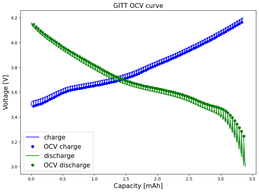
To plot our results, we additionally get the entire voltage vs capacity curves for the selected GITT cycle, employing the .get_ccap and .get_dcap methods. The cell mass is used to convert from gravimetric capacity (mAh/g) to capacity (mAh).

c.make_step_table(all_steps=False)
ccap = c.get_ccap(cycle=GITT_cycle)
dcap = c.get_dcap(cycle=GITT_cycle)
mass = c.get_mass() # in mg

fig, ax = plt.subplots()
ax.plot(ccap["charge_capacity"]*mass/1000, ccap["voltage"], color='blue', label="charge")
ax.plot(cap_cha, V_cha, "bo", label="OCV charge")
ax.plot(dcap["discharge_capacity"]*mass/1000, dcap["voltage"], color="green", label="discharge")
ax.plot(cap_dch, V_dch, "go", label="OCV discharge")
plt.xlabel("Capacity [mAh]", fontsize=15)
plt.ylabel("Voltage [V]", fontsize=15)
plt.title("GITT OCV curve", fontsize=15)
#plt.ylim(0, 0.91)
#plt.xlim(0, 4.70)
ax.legend(fontsize=15)
fig.set_figheight(7)
fig.set_figwidth(10)
plt.show()

Saving the data

Concatenate the OCV voltages and capacities into a dataframe, and save as a .csv file.

OCV_cha = pd.concat([cap_cha, V_cha], axis=1 ,keys=["Charge_cap_mAh","OCV_V"])
OCV_dch = pd.concat([cap_dch, V_dch], axis=1, keys=["Discharge_cap_mAh", "OCV_V"])

#OCV_cha.to_csv('GITT_OCV_cycle'+str(GITT_cycle)+'_cha.csv', index=False)
#OCV_dch.to_csv('GITT_OCV_cycle'+str(GITT_cycle)+'_dch.csv', index=False)