Using some of the cellpy special utilities

Open Circuit Relaxation

Note

This chapter would benefit from some more love and care. Any help on that would be highly appreciated.

Plotting selected Open Circuit Relaxation points

# assuming b is a cellpy.utils.batch.Batch object

from cellpy.utils.batch_tools.batch_analyzers import OCVRelaxationAnalyzer
# help(OCVRelaxationAnalyzer)

print(" analyzing ocv relaxation data ".center(80, "-"))
analyzer = OCVRelaxationAnalyzer()
analyzer.assign(b.experiment)
analyzer.direction = "down"
analyzer.do()
dfs = analyzer.last
df_file_one, _df_file_two = dfs

# keeping only the columns with voltages
ycols = [col for col in df_file_one.columns if col.find("point")>=0]

# removing the first ocv rlx (relaxation before starting cycling)
df = df_file_one.iloc[1:, :]
# tidy format
df = df.melt(
    id_vars = "cycle", var_name="point", value_vars=ycols,
    value_name="voltage"
)

# using holoviews for plotting
curve = hv.Curve(
    df, kdims=["cycle", "point"],
    vdims="voltage"
).groupby("point").overlay().opts(xlim=(1,10), width=800)

Open Circuit Relaxation modeling

TODO.

Extracting ica data

Note

This chapter would benefit from some more love and care. Any help on that would be highly appreciated.

Example: get dq/dv data for selected cycles

This example shows how to get dq/dv data for a selected cycle. The data is extracted from the cellpy object using the .get_cap method. The method dqdv_cycle and the dqdv methods are cellpy-agnostic and should work also for other data sources (e.g. numpy arrays).

import matplotlib.pyplot as plt
from cellpy.utils import ica

v4, dqdv4 = ica.dqdv_cycle(
    data.get_cap(
        4,
        categorical_column=True,
        method = "forth-and-forth")
)

v10, dqdv10 = ica.dqdv_cycle(
    data.get_cap(
        10,
        categorical_column=True,
        method = "forth-and-forth")
)

plt.plot(v4,dqdv4, label="cycle 4")
plt.plot(v10, dqdv10, label="cycle 10")
plt.legend()

Example: get dq/dv data for selected cycles

This example shows how to get dq/dv data directly from the cellpy object. This methodology is more convenient if you want to get the data easily from the cellpy object in a pandas dataframe format.

# assuming that b is a cellpy.utils.batch.Batch object

c = b.experiment.data["20160805_test001_45_cc"]  # get the cellpy object
tidy_ica = ica.dqdv_frames(c)  # create the dqdv data
cycles = list(range(1,3)) + [10, 15]
tidy_ica = tidy_ica.loc[tidy_ica.cycle.isin(cycles), :]  # select cycles

Fitting ica data

TODO.

Using the batch utilities

The steps given in this tutorial describes how to use the new version of the batch utility. The part presented here is chosen such that it resembles how the old utility worked. However, under the hood, the new batch utility is very different from the old. A more detailed guide will come soon.

So, with that being said, here is the promised description.

Starting (setting things up)

A database

Currently, the only supported “database” is Excel (yes, I am not kidding). So, there is definitely room for improvements if you would like to contribute to the code-base.

The Excel work-book must contain a page called db_table. And the top row of this page should consist of the correct headers as defined in your cellpy config file. You then have to give an identification name for the cells you would like to investigate in one of the columns labelled as batch columns ( typically “b01”, “b02”, …, “b07”). You can find an example of such an Excel work-book in the test-data.

A tool for running the job

Jupyter Notebooks is the recommended “tool” for running the cellpy batch feature. The first step is to import the cellpy.utils.batch.Batch class from cellpy. The Batch class is a utility class for pipe-lining batch processing of cell cycle data.

from cellpy.utils import batch, plotutils
from cellpy import prms
from cellpy import prmreader

The next step is to initialize it:

project = "experiment_set_01"
name = "new_exiting_chemistry"  # the name you set in the database
batch_col = "b01"
b = batch.init(name, project, batch_col=batch_col)

and set some parameters that Batch needs:

# setting additional parameters if the defaults are not to your liking:
b.experiment.export_raw = True
b.experiment.export_cycles = True
b.experiment.export_ica = True
b.experiment.all_in_memory = True  # store all data in memory, defaults to False
b.save_cellpy_file = True

b.force_raw_file = False
b.force_cellpy_file = True

Extracting meta-data

The next step is to extract and collect the information needed from your data-base into a DataFrame, and create an appropriate folder structure (outdir/project_name/batch_name/raw_data)

# load info from your db and write the journal pages
b.create_journal()
b.create_folder_structure()

Processing data

To run the processing, you should then use the convenience function update. This function loads all your data-files and saves csv-files of the results.

b.update()

The next step is to create some summary csv-files (e.g. containing charge capacities vs. cycle number for all your data-files) and plot the results.

b.make_summaries()
b.plot_summaries()

Now it is time to relax and maybe drink a cup of coffee.

Further investigations and analyses

There are several paths to go from here. I recommend looking at the raw data for the different cells briefly to check if everything looks sensible. You can get the names of the different datasets (cells) by issuing:

b.experiment.cell_names

You can get the CellpyCell-object for a given cell by writing:

cell = b.experiment.data[name_of_cell]
plotutils.raw_plot(my_cell)

If you want to investigate further, you can either use one of the available analysis-engines (they work on batch objects processing all the cells at once) or you can continue on a single cell basis (latter is currently recommended).

Another tip is to make new Notebooks for each type of “investigation” you would like to perform. You can load the info-df-file you created in the initial steps, or you could load the individual cellpy-files (if you did not turn off automatic saving to cellpy-format).

You should be able to find examples of processing either by downloading the examples or by looking in the repo.

Collectors

Todo.

Have a look at the data

Note

This chapter would benefit from some more love and care. Any help on that would be highly appreciated.

Here are some examples how to get a peak at the data. If we need an interactive plot of the raw-data, we can use the plotutils.raw_plot function. If we would like to see some statistics for some of the cycles, the plotutils.cycle_info_plot is your friend. Let´s start by importing cellpy and the plotutils utility:

import cellpy
from cellpy.utils import plotutils

Let´s load some data first:

cell = cellpy.get("../testdata/hdf5/20160805_test001_45_cc.h5", mass=0.8)

Here we used the convenience method cellpy.get to load some example data. If everything went well, you will see an output approximately like this:

(cellpy) - Making CellpyCell class and setting prms
(cellpy) - Loading cellpy-file: ../testdata/hdf5/20160805_test001_45_cc.h5
(cellpy) - Setting mass: 0.8
(cellpy) - Creating step table
(cellpy) - Creating summary data
(cellpy) - assuming cycling in anode half-cell (discharge before charge) mode
(cellpy) - Created CellpyCell object

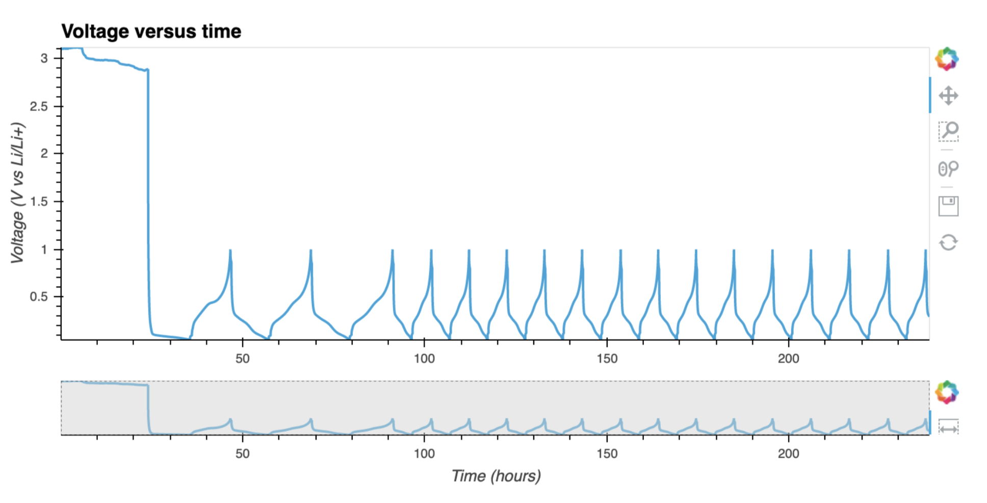
If you have holoviews installed, you can conjure an interactive figure:

plotutils.raw_plot(cell)

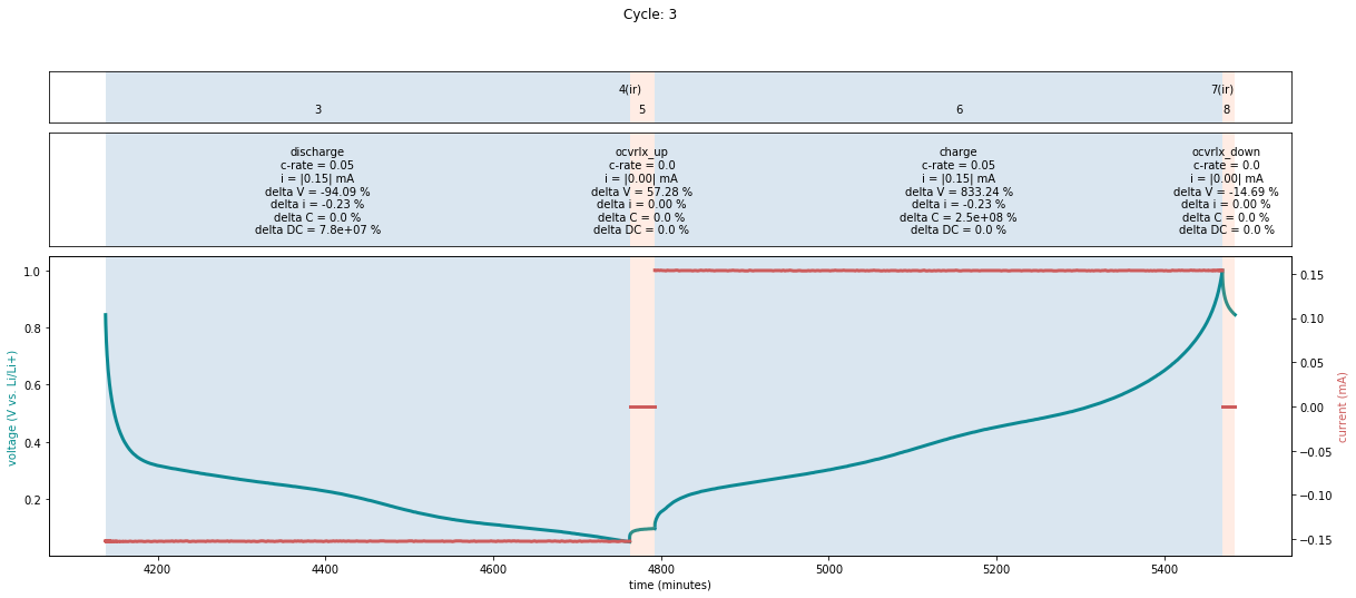
Sometimes it is necessary to have a look at some statistics for each cycle and step. This can be done using the cycle_info_plot method:

fig = plotutils.cycle_info_plot(
    cell,
    cycle=3,
    use_bokeh=False,
)

Note

If you chose to work within a Jupyter Notebook, you are advised to try some of the web-based plotting tools. For example, you might consider installing holoviz suite.

Easyplot

Todo.

Templates

Note

This chapter would benefit from some more love and care. Any help on that would be highly appreciated.

Some info can be found in one of the example notebooks (Example notebooks). It would be more logical if that information was here instead. Sorry for that.

Custom loaders

Todo.